Version 1.2.1 · 16 August 2026 · Micah Forstein
Also available as a typeset PDF for printing or circulation.
Changes in 1.2.1: the remedy for a collapsed scale now takes effect when it is switched on, rather than at the next file load; the on-screen warning no longer covers the values it describes; and this document gains a pipeline overview, a glossary, and figures for the results that were previously stated only in prose.
Changes in 1.2.0: scaling that has collapsed input columns is now detected and reported before any score (Section 2.4). Found by a user comparing the raw and scaled rows on screen — six distinct inputs were arriving at the engine as one value, and every error figure agreed with itself while describing a model with a fifth of the inputs the file contained.
Changes in 1.1.0: ensemble members may now be defined by the user (Section 6.6), which widens what the agreement check measures from initialisation sensitivity to specification sensitivity, and adds a comparability test between members.
This document specifies every calculation the software performs, in enough detail to reimplement it. It is written for someone who validates models: the intent is that a reader can check the claims rather than take them, and can see precisely where each figure in the model card comes from.
Section 9 is the one that matters most. It states what these methods cannot establish. A validation layer that only lists its strengths is doing the same thing it exists to catch.
How to read this document. The two unnumbered sections that follow are orientation: a map of the whole procedure, and the vocabulary it uses. Neither contains anything that is not stated more precisely later, so a reader who wants the specification alone can begin at Section 1 and lose nothing. Sections 1 through 8 are the specification. Section 9 is the limitations, Section 10 the defaults, and Section 11 the commands that reproduce every figure quoted here.
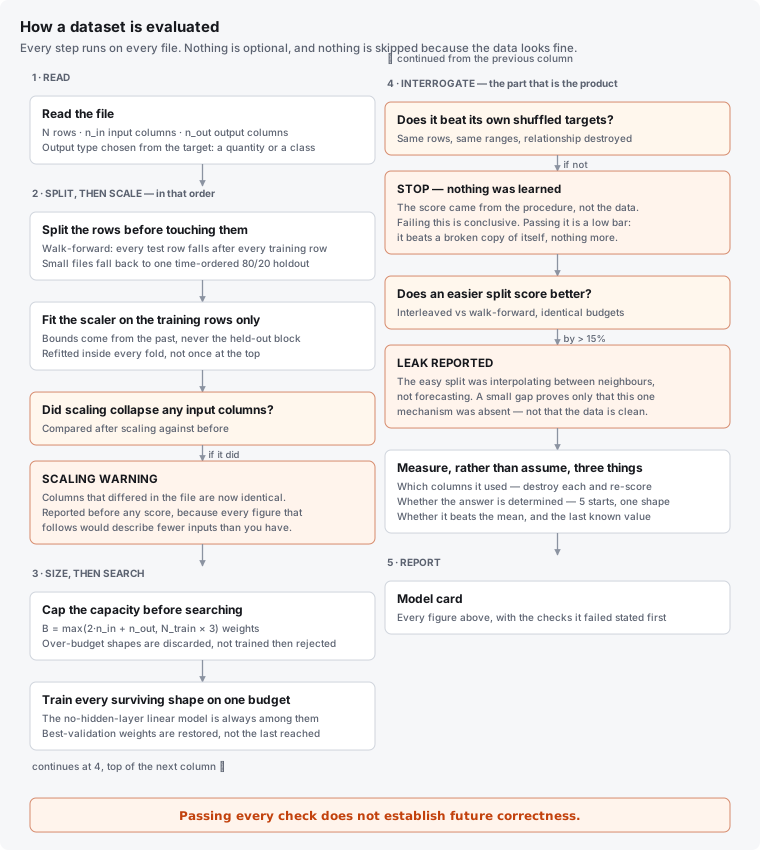
Every file takes the same path, in the same order. The order is not an implementation detail: several of these steps are only valid because of what precedes them, and performing them in a different sequence produces figures that are internally consistent and wrong.
Three features of that diagram carry most of the argument.
Splitting comes before scaling, and scaling comes before everything else. Column bounds are learned from the training rows alone (Section 2.5). Fitting them on the whole file first would let the held-out rows contribute their own minimum and maximum, so the model would know the range of data it is about to be tested on. The resulting score is optimistic by an amount nobody can estimate after the fact, and nothing in the output looks wrong.
Capacity is bounded before the search begins, not after. Shapes that exceed the weight budget are discarded without being trained (Section 5.1). A network with more parameters than the data can constrain will fit the training rows beautifully, and rejecting it on its held-out score afterwards means the search has already spent its budget exploring models that could never have been kept.
Two of the checks can only ever return bad news. The negative control (Section 6.4) and the leak indicator (Section 6.3) are one-sided. Failing either settles the question: the score came from the procedure rather than the data, or the easy split was flattering it. Passing them settles nothing, because the conditions they test are a small subset of the ways a result can be wrong. That asymmetry is drawn deliberately: in Figure 1 each is a question followed by the single finding it can return, an exit from the sequence rather than a milestone along it.
The terms below are used throughout with these specific meanings. Where a term is in general use with a looser sense, the narrower reading is the one intended here.
| Term | Meaning |
|---|---|
| Row / case | One observation: a vector of inputs paired with the answer for that observation. |
| Column | One variable measured across every row. Input columns are what the model may use; output columns are what it must predict. |
| Training partition | The rows the model is allowed to learn from, and the only rows from which any quantity — including scaling bounds — may be derived. |
| Held-out / test partition | Rows deliberately withheld from training, used once to score the result. A row used to choose the model is no longer held out. |
| Fold | One train/test division. Several folds give several independent scores instead of one lucky or unlucky number. |
| Walk-forward split | A split where every test row falls after every training row in time. The only honest arrangement for sequential data. |
| Interleaved split | A split holding out every $k$th row, scattered through the series. Valid for exchangeable rows, and misleading for sequential ones (Section 6.2). |
| Leakage | Any route by which information unavailable at prediction time reaches the model during training. Its signature is a score that is too good and cannot be reproduced in use. |
| Term | Meaning |
|---|---|
| Scaling / normalisation | Mapping each column onto a common interval so no column dominates through its units alone. Here, min–max scaling (Section 2.1). |
| Per-column scaling | Each column scaled on its own observed range. Correct when columns are different quantities. |
| Shared input scale | Every input column scaled on one common range. Correct when the columns are the same quantity repeated — lags of a series, or several readings from one sensor. |
| Collapse | The failure in which per-column scaling maps genuinely different columns onto identical values, destroying the offsets that distinguished them (Section 2.4). |
| Target band | The interval $[0.1, 0.9]$ into which output targets are mapped, so no target sits on a value a logistic node cannot reach (Section 2.2). |
| Saturation | A sigmoid driven so far toward 0 or 1 that its gradient is effectively zero. A saturated node stops learning and does not recover on its own. |
| Term | Meaning |
|---|---|
| Shape / architecture | The widths of the layers, written $s_0 \rightarrow s_1 \rightarrow \cdots \rightarrow s_\Lambda$. |
| Weight | One trainable number on one connection. The count of them is the model's capacity (Section 3.3). |
| Iteration | One full pass over the training rows. Not one weight update: a pass over $N$ rows performs $N$ updates. |
| Learning rate $\eta$ | How far each update moves a weight. |
| Momentum $\mu$ | The fraction of the previous update carried into the current one. It accelerates consistent descent and amplifies the effective step by $1/(1-\mu)$, which is why a step cap is required (Section 4.4). |
| Weight decay $\lambda$ | A constant shrinkage applied to every weight each step, restraining unbounded growth. |
| Capacity budget | A ceiling on the weight count derived from the number of training rows, applied before the search (Section 5.1). |
| Term | Meaning |
|---|---|
| Baseline | A deliberately unintelligent prediction the model must beat to be worth anything: the training mean, or the last known value. |
| MSE / MAE | Mean squared error, used for ranking candidates; mean absolute error, reported in the user's own units because it can be interpreted (Section 6.7). |
| Negative control | The same model trained on the same data with the targets shuffled, so every real relationship is destroyed and every structural property is kept (Section 6.4). |
| Permutation importance | How much the score worsens when one input column is scrambled — a measurement of what the model used, not of what causes what (Section 6.5). |
| Ensemble spread | The disagreement among several networks trained on identical data from different starting points. It measures whether the answer is determined, not whether it is right (Section 6.6). |
| Prequential evaluation | Scoring a stream by predicting each case before training on it, so no prediction can use information from its own future (Section 7). |
| Symbol | Meaning |
|---|---|
| $N$ | Number of rows (cases) in a dataset. |
| $n_{\mathrm{in}}$, $n_{\mathrm{out}}$ | Input and output column counts. |
| $\mathbf{x}\in\mathbb{R}^{n_{\mathrm{in}}}$ | One row's input vector, in real units. |
| $\mathbf{y}\in\mathbb{R}^{n_{\mathrm{out}}}$ | That row's target vector, in real units. |
| $\tilde{\mathbf{x}},\ \tilde{\mathbf{y}}$ | The same vectors after scaling (Section 2). |
| $L$ | Layer index, with $L=0$ the input layer and $L=\Lambda$ the output layer. |
| $s_L$ | Width of layer $L$, so $s_0=n_{\mathrm{in}}$ and $s_\Lambda=n_{\mathrm{out}}$. |
| $a_j^{(L)}$ | Activation of node $j$ in layer $L$. |
| $w_{jk}^{(L)}$ | Weight into node $j$ of layer $L+1$ from node $k$ of layer $L$. |
| $b_j^{(L)}$ | Bias weight of node $j$ in layer $L+1$. |
| $\delta_j^{(L)}$ | Error signal at node $j$ of layer $L$. |
| $\eta$ | Learning rate, default $0.5$. |
| $\mu$ | Momentum, default $0.9$. |
| $\lambda$ | Weight decay, default $0$. |
| $\beta$ | Bias activation constant, $0.5$. |
A network shape is written
$$s_0 \rightarrow s_1 \rightarrow \cdots \rightarrow s_\Lambda,$$
for example
$$30 \rightarrow 36 \rightarrow 30 \rightarrow 15 \rightarrow 6.$$
Raw columns are on incompatible scales — dollars beside counts beside degrees. A sigmoid responds usefully only over a limited input range, so every column is mapped onto a common interval before training.
In plain terms: the engine cannot see units. A column of share prices in the thousands and a column of counts in single figures are, to the arithmetic, simply large numbers and small ones, and the large ones will dominate for no reason beyond how they happen to be denominated. Scaling puts every column on a common footing first. The three subsections that follow are the three decisions that involves: what range to use, where to put the answers, and how to get back to real units afterwards. Section 2.4 is the case where the obvious choice is wrong.
For input column $c$, let $\ell_c$ and $h_c$ be the minimum and maximum observed in the training partition only. Then
$$\boxed{\ \tilde{x}_c = \frac{x_c - \ell_c}{h_c - \ell_c}\ } \tag{2.1}$$
A constant column satisfies $h_c = \ell_c$. It carries no information and would divide by zero, so it is mapped to
$$\tilde{x}_c = 0.5.$$
An earlier implementation derived one global minimum and maximum across all inputs and outputs. On aatrainingdata.csv (inputs 1–40, outputs 21–225) that compressed every input into $[0.004, 0.178]$, forcing the network to resolve six inputs inside 18% of its usable range. Per-column scaling measured approximately 2.2× lower error on that file at equal iteration count.
Output columns are mapped not to $[0,1]$ but to
$$[\tau_{\mathrm{lo}}, \tau_{\mathrm{hi}}] = [0.1,\ 0.9].$$
First normalise each output column:
$$u_c = \frac{y_c - y_c^{\min}}{y_c^{\max} - y_c^{\min}}.$$
Then map the normalised value into the target band:
$$\boxed{\ \tilde{y}_c = \tau_{\mathrm{lo}} + (\tau_{\mathrm{hi}} - \tau_{\mathrm{lo}})\,u_c\ } \tag{2.2}$$
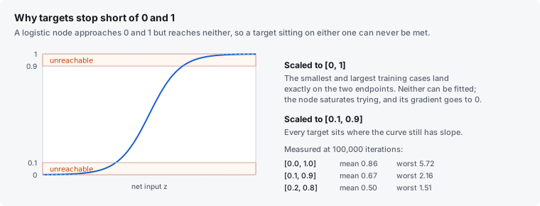
The reason is structural. A logistic output node emits values in the open interval $(0,1)$; it approaches $0$ and $1$ asymptotically and reaches neither. Under $[0,1]$ scaling the smallest and largest training cases land exactly on the two unreachable endpoints, so those two cases can never be fitted and the node saturates while attempting it.
Measured on aatrainingdata.csv at 100,000 iterations:
| Target band | Mean error | Worst error |
|---|---|---|
| $[0.0, 1.0]$ | 0.86 | 5.72 |
| $[0.1, 0.9]$ | 0.67 | 2.16 |
| $[0.2, 0.8]$ | 0.50 | 1.51 |
Inputs are left on $[0,1]$, since nothing is required to reproduce them.
The narrower the band, the lower the measured error — which invites the question of why the band is not narrower still. Compressing the targets shrinks the differences the network is being asked to resolve, and past some point the model is accurate about a range so small it is no longer saying much. $[0.1, 0.9]$ keeps the extremes off the asymptotes while leaving 80% of the output range in use.
Predictions are returned to real units by reversing the target-band transformation. First,
$$u_c = \frac{\hat{y}_{c,\mathrm{scaled}} - \tau_{\mathrm{lo}}}{\tau_{\mathrm{hi}} - \tau_{\mathrm{lo}}}.$$
Then
$$\boxed{\ \hat{y}_c = u_c\,(y_c^{\max} - y_c^{\min}) + y_c^{\min}\ } \tag{2.3}$$
Every error figure reported in real units passes through this inverse transform first, so it is denominated in the units of the user's own data.
When input columns are the same quantity repeated — lags of one series, or six readings from one sensor — per-column scaling is actively wrong. Consider a ramp where column $c$ holds $i + c - 1$. Per-column scaling subtracts a different minimum from each column:
$$\frac{(i + c - 1) - c}{\mathrm{span}} = \frac{i - 1}{\mathrm{span}}. \tag{2.4}$$
The column index $c$ cancels. All columns collapse to one repeated value, and the offsets that distinguished them are destroyed. Setting sharedInputScale puts every input column on one ruler — the widest bound observed across any of them — preserving inter-column differences.
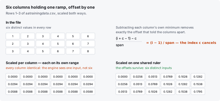
The failure is worth dwelling on because of how it presents. Nothing errors, nothing is obviously missing, and the error figures that follow are all correctly computed — of a model with one input rather than six. A reader checking the output for signs of trouble will not find any. The only visible symptom is a row of identical numbers on the canvas, which is why the software now says so directly rather than relying on it being noticed.
This condition is now detected and reported rather than left to be noticed. After fitting, the scaler compares every input column against each earlier one and flags any that became identical after scaling while differing before it. That distinction matters: a column that was always a copy carried no information to lose, whereas one made identical by scaling has had information destroyed.
The check is reported before any score, because every figure that follows would have been computed on fewer inputs than the file appears to contain. On aatrainingdata.csv, six columns holding a ramp offset by one each collapse to a single value, and the engine reports that it is seeing one distinct input rather than six. On the shipped sample files with genuine multi-column structure the check stays silent, including leak_demo.csv, whose lag columns are noisy enough that they do not collapse exactly.
As of 1.2.1 the remedy takes effect when it is selected. Enabling the shared scale discards any rows already scaled the other way and re-evaluates the condition immediately, so the reported state and the values on screen both change at the moment of the change. Previously the flag was recorded but the scaled rows were cached, and the setting appeared to do nothing until the file was loaded again — a diagnosis pointing at a remedy that did not visibly work is worse than no diagnosis, because it also spends the reader's trust in the diagnosis.
Scaler.fit() is called on the training partition alone, and the resulting instance is applied unchanged to the test partition. Fitting bounds on the full dataset would leak the test set's range into training: the model would know the future's minimum and maximum. This is a common and near-invisible source of optimistic bias, and it is why the scaler is refitted inside every fold rather than once at the top.
In plain terms: a layer takes the numbers below it, multiplies each by a weight, adds them up, and squashes the total into a bounded range. Repeating that with several layers is the whole model. The three subsections cover how a value moves forward through it (3.1), what the weights start as and why that choice is not arbitrary (3.2), and how to count them, since the count is what Section 5 later constrains (3.3).
Layers are fully connected. For $L = 0,\ldots,\Lambda-1$, the net input to node $j$ in layer $L+1$ is
$$\boxed{\ z_j^{(L+1)} = \beta b_j^{(L)} + \sum_{k=1}^{s_L} w_{jk}^{(L)} a_k^{(L)}\ } \tag{3.1}$$
The bias term is a weight multiplied by a constant activation $\beta = 0.5$, rather than the more usual $1$. This reproduces the behaviour of the original 1993 engine's ballast node and is retained so that results remain comparable across the rewrite. It is mathematically equivalent to a bias of $b/2$ with unit activation; only the effective learning rate on the bias differs.
Activation is logistic everywhere except, optionally, at the output:
$$\boxed{\ \sigma(z) = \frac{1}{1 + e^{-z}}\ } \tag{3.2}$$
Thus hidden layers use
$$a_j^{(L+1)} = \sigma\!\left(z_j^{(L+1)}\right),$$
while the output layer is
$$a_j^{(\Lambda)} = \begin{cases} z_j^{(\Lambda)}, & \text{linear output (regression)},\\[4pt] \sigma\!\left(z_j^{(\Lambda)}\right), & \text{sigmoid output (classification)}. \end{cases}$$
Why a linear output matters. The sigmoid's asymptotes (Section 2.2) mean a regression target at either extreme is unreachable, which is why the largest case in a regression file is reliably the worst predicted. A linear output removes the ceiling entirely, so targets may use their full range and the extremes stop being special. Sigmoid remains correct for classification, where outputs are intended as probabilities in $(0,1)$.
The output type is chosen automatically from the target column's character and can be forced with --linear or --sigmoid.
Weights are drawn from Glorot (Xavier) uniform initialisation:
$$\boxed{\ w_{jk}^{(L)} \sim \mathcal{U}(-r_L, +r_L), \qquad r_L = \sqrt{\frac{6}{s_L + s_{L+1}}}\ } \tag{3.3}$$
with
$$b_j^{(L)} = 0.$$
A node's net input is a sum of $s_L$ weighted terms. With a fixed spread, the variance of that sum grows with layer width, so a wide layer begins deep in the sigmoid's flat tails. A saturated sigmoid has gradient $\sigma(1-\sigma) \approx 0$ and therefore never recovers. This was measured as a completely dead hidden layer in 4 of 10 streaming runs before (3.3) was adopted. Scaling by $\sqrt{6/(\mathrm{fan\_in} + \mathrm{fan\_out})}$ holds the net input near unit variance regardless of width, which is where the sigmoid actually has slope.
Biases start at zero: training moves them where needed, and a nonzero start is an unmotivated prior.
The total number of trainable parameters is
$$\boxed{\ W(\mathbf{s}) = \sum_{L=0}^{\Lambda-1}\left(s_L s_{L+1} + s_{L+1}\right)\ } \tag{3.4}$$
Equivalently,
$$W(\mathbf{s}) = \underbrace{\sum_{L=0}^{\Lambda-1} s_L s_{L+1}}_{\text{connection weights}} \;+\; \underbrace{\sum_{L=0}^{\Lambda-1} s_{L+1}}_{\text{bias weights}}.$$
This is the quantity constrained by the capacity budget in Section 5.
In plain terms: show the network a row, compare its answer to the truth, and push every weight a little way in the direction that would have made the answer better. Repeat. Everything below that simple loop is guarding against the two ways it destroys itself — a single extreme case throwing the weights so far that the sigmoids stop responding (4.2–4.4), and weights growing without limit until the network becomes a bank of step functions (4.4). Sections 4.5 and 4.6 recover what can be recovered when it happens anyway.
Per case, the objective is one-half squared error summed over outputs:
$$\boxed{\ E = \frac{1}{2}\sum_{j=1}^{n_{\mathrm{out}}}\left(a_j^{(\Lambda)} - \tilde{y}_j\right)^2\ } \tag{4.1}$$
Optimisation is stochastic, per-sample gradient descent: weights are updated after every case, not after a batch. One iteration is one full pass over the training rows, so a run of $T$ iterations over $N$ rows performs
$$N_{\mathrm{updates}} = TN$$
updates.
Using
$$\sigma'(z) = \sigma(z)\left(1 - \sigma(z)\right),$$
the output-layer error signal is
$$\delta_j^{(\Lambda)} = \begin{cases} \left(a_j^{(\Lambda)} - \tilde{y}_j\right) a_j^{(\Lambda)}\left(1 - a_j^{(\Lambda)}\right), & \text{sigmoid output},\\[6pt] \left(a_j^{(\Lambda)} - \tilde{y}_j\right), & \text{linear output}. \end{cases} \tag{4.2}$$
Delta clipping. With a sigmoid output, $|\delta| \le 0.25$ automatically because $o(1-o) \le 1/4$. The factor is self-limiting. A linear output discards it, leaving the raw difference, which is unbounded. On a live feed the first prediction can be extreme — one measured instance produced 702 against a target of 17. A single step of that magnitude drives the hidden weights so far negative that their sigmoids sit at zero for every input; the layer is then dead, no gradient flows back through it, and it never recovers. Therefore
$$\boxed{\ \delta_j^{(\Lambda)} \leftarrow \mathrm{clip}\!\left(\delta_j^{(\Lambda)}, -\Delta, +\Delta\right), \qquad \Delta = 1.0\ } \tag{4.3}$$
with $\Delta = 0$ disabling clipping.
Backwards for $L = \Lambda-1, \ldots, 1$,
$$\boxed{\ \delta_k^{(L)} = \left(\sum_j w_{jk}^{(L)} \delta_j^{(L+1)}\right) a_k^{(L)}\left(1 - a_k^{(L)}\right)\ } \tag{4.4}$$
which separates visually into
$$\underbrace{a_k^{(L)}\left(1 - a_k^{(L)}\right)}_{\text{local sigmoid gradient}} \times \underbrace{\sum_j w_{jk}^{(L)} \delta_j^{(L+1)}}_{\text{error arriving from the next layer}}.$$
Each node's error is the weighted sum of the errors it feeds, times its own sigmoid slope. All $\delta$ values are computed before any weight is modified, so (4.4) reads pre-update weights throughout. Updating in place mid-pass would corrupt the gradient of the layers below.
For each connection,
$$v_{jk}^{(L)} \leftarrow \mathrm{clip}\!\left(-\eta\,\delta_j^{(L+1)} a_k^{(L)} + \mu v_{jk}^{(L)},\ -S,\ +S\right),$$
$$w_{jk}^{(L)} \leftarrow w_{jk}^{(L)} + v_{jk}^{(L)} - \lambda w_{jk}^{(L)}. \tag{4.5}$$
For each bias,
$$v_{b,j}^{(L)} \leftarrow \mathrm{clip}\!\left(-\eta\,\delta_j^{(L+1)}\beta + \mu v_{b,j}^{(L)},\ -S,\ +S\right),$$
$$b_j^{(L)} \leftarrow b_j^{(L)} + v_{b,j}^{(L)} - \lambda b_j^{(L)},$$
with default per-step cap $S = 1.0$, and $S = 0$ disabling the cap.
Equivalently, the weight update may be read as
$$w_{jk}^{(L)} \leftarrow (1-\lambda)\,w_{jk}^{(L)} + v_{jk}^{(L)},$$
which makes the shrinkage due to weight decay explicit: every update multiplies the old weight by $1-\lambda$.
Why momentum needs a step cap. Under a sustained gradient $g$, the velocity recursion is
$$v_t = -\eta g + \mu v_{t-1},$$
so at equilibrium $v_\infty = -\eta g + \mu v_\infty$, giving
$$\boxed{\ v_\infty = -\frac{\eta g}{1 - \mu}\ } \tag{4.6}$$
At $\mu = 0.9$,
$$\frac{1}{1-\mu} = \frac{1}{0.1} = 10,$$
a ten-fold amplification of the nominal learning rate. Clipping $\delta$ alone is insufficient, because hidden deltas are that delta multiplied by the weights above them. Once a weight is large, the resulting step is large again. Bounding the step itself bounds the damage any single sample can do.
Weight decay. The $-\lambda w$ term is an $L_2$ pull toward zero applied per step. Without it nothing prevents unbounded weight growth: one measured run on a drifting feed reached a bias of 44 and weights of 21, which put every hidden sigmoid hard against 0 or 1. They became step functions, and the output swung to 1648 against targets of 10–80.
Decay is off by default, and the reason is arithmetic. Because it applies per step, its total effect depends on the number of steps taken. Batch training in the GUI performs on the order of 560,000 steps, where even $\lambda = 10^{-5}$ compounds to
$$\boxed{\ \left(1 - 10^{-5}\right)^{560\,000} \approx 0.0037\ } \tag{4.7}$$
leaving roughly $0.37\%$ of the original magnitude — shrinking the weights to essentially nothing, measured as held-out error rising from 0.41 to 1.74. Batch training has early stopping and a validation set to keep it honest. A live feed has neither, so streaming mode enables decay for itself while batch mode leaves it off.
A sigmoid saturated at 0 or 1 has gradient $\sigma(1-\sigma) = 0$, receives no correction, and remains stuck permanently. No amount of further gradient descent recovers it. The only remedy is to place the node somewhere it has slope again, so reinitIncoming redraws that node's incoming weights from (3.3) and clears its momentum. Layers above keep their weights; the network loses only that node's contribution.
Training error does not decrease monotonically, and the final iteration is rarely the best on unseen data. The trainer snapshots weights at the best validation score and restores them at the end, so the network kept is the best one found rather than the last one reached.
The dominant failure mode for a small dataset is a network with more parameters than the data can constrain. Capacity is bounded before the search begins.
The budget is
$$\boxed{\ B = \max\!\left(2n_{\mathrm{in}} + n_{\mathrm{out}},\ N_{\mathrm{train}}\,\rho\right), \qquad \rho = 3\ } \tag{5.1}$$
where $\rho$ is the number of weights permitted per training row (--weights-per-row). Any candidate shape satisfying
$$W(\mathbf{s}) > B$$
is discarded outright rather than trained and rejected.
The search enumerates a fixed family rather than a random or exhaustive one. Define
$$h_{\mathrm{base}} = \max\!\left(2,\ \mathrm{round}\sqrt{n_{\mathrm{in}} n_{\mathrm{out}}} + 1\right),$$
the geometric mean of input and output width, rounded and offset by one. Candidates are:
Duplicates and over-budget shapes are dropped. The no-hidden-layer shape is always included and always reported: it is a linear model, and if it is competitive then the nonlinearity is not earning its place.
Every quantity in Sections 3.3, 5.1, 5.2 and 5.3 can be checked by hand on one file. For aatrainingdata.csv: $n_{\mathrm{in}} = 6$, $n_{\mathrm{out}} = 1$, $N = 35$, of which $N_{\mathrm{train}} = 33$ after the hold-out.
The budget, from (5.1):
$$B = \max(2 \cdot 6 + 1,\ 33 \cdot 3) = \max(13,\ 99) = 99.$$
The hidden width, from Section 5.2:
$$h_{\mathrm{base}} = \max\!\left(2,\ \mathrm{round}\sqrt{6 \cdot 1} + 1\right) = \max(2,\ 3) = 3,$$
giving $h \in \{3, 6, 7, 12\}$ after removing the duplicate produced by $n_{\mathrm{in}}/2 = 3$. Enumerating the four families yields twelve candidates. Applying (3.4) to each and discarding those above $B$:
| Shape | $W(\mathbf{s})$ | Kept |
|---|---|---|
| $6 \rightarrow 1$ | 7 | yes |
| $6 \rightarrow 3 \rightarrow 1$ | 25 | yes |
| $6 \rightarrow 6 \rightarrow 1$ | 49 | yes |
| $6 \rightarrow 7 \rightarrow 1$ | 57 | yes |
| $6 \rightarrow 12 \rightarrow 1$ | 97 | yes |
| $6 \rightarrow 3 \rightarrow 2 \rightarrow 1$ | 32 | yes |
| $6 \rightarrow 3 \rightarrow 3 \rightarrow 1$ | 37 | yes |
| $6 \rightarrow 6 \rightarrow 4 \rightarrow 1$ | 75 | yes |
| $6 \rightarrow 6 \rightarrow 6 \rightarrow 1$ | 91 | yes |
| $6 \rightarrow 7 \rightarrow 4 \rightarrow 1$ | 86 | yes |
| $6 \rightarrow 7 \rightarrow 7 \rightarrow 1$ | 113 | no — over budget |
| $6 \rightarrow 7 \rightarrow 6 \rightarrow 3 \rightarrow 1$ | 122 | no — over budget |
Ten shapes survive. The iteration budget, from (5.2):
$$T = \max\!\left(400,\ \min\!\left(6000,\ \left\lfloor \tfrac{150\,000}{33} \right\rfloor\right)\right) = 4545.$$
Running DetectBS --auto --in data/aatrainingdata.csv reports a weight budget of 99, ten shapes to try, and a search at 4545 iterations each, with the per-shape weight counts above. The equations in this document and the shipped program agree because they are the same arithmetic; the point of stating both is that a reader can confirm it without reading the source.
When iterations are not specified,
$$\boxed{\ T = \max\!\left(400,\ \min\!\left(6000,\ \frac{150\,000}{N_{\mathrm{train}}}\right)\right)\ } \tag{5.2}$$
What matters is how many times each case is seen, not the iteration count. A fixed 6000 iterations is seconds on 28 rows and minutes on 600, for no additional benefit.
This is the part of the software that distinguishes it. Everything above is a competent but unremarkable backpropagation engine.
In plain terms: everything up to here produces a number. This section is about whether the number means anything. The four checks answer four different questions, and it is worth keeping them apart. Section 6.1–6.3 ask whether the score was obtained honestly. Section 6.4 asks whether anything was learned at all. Section 6.5 asks what the model actually used. Section 6.6 asks whether the answer was determined by the data or by where the optimiser happened to start. A model can pass any one of them and fail the rest.
For sequential data, the only honest split trains on the past and tests on the future. With $N$ rows and $F$ folds,
$$N_{\mathrm{test,total}} = \max\!\left(F,\ \left\lfloor \frac{N}{4} \right\rfloor\right), \qquad b = \max\!\left(1,\ \left\lfloor \frac{N_{\mathrm{test,total}}}{F} \right\rfloor\right),$$
and
$$s = N - bF.$$
For fold $f$,
$$\mathrm{cut}_f = s + fb,$$
with training rows $[0, \mathrm{cut}_f)$ and test rows $[\mathrm{cut}_f, \mathrm{end}_f)$, where $\mathrm{end}_f = \mathrm{cut}_f + b$, except that the last fold ends at $N$.
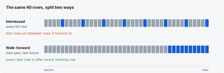
The training window expands; the test block always sits immediately after it. The final fold is the closest available analogue to how the model would really be used. Each fold refits its own scaler (Section 2.5).
The central ordering condition is
$$\boxed{\ \max(\text{training time}) < \min(\text{test time})\ }$$
which is the mathematical statement of no future data in the training set.
Three degenerate cases fall back to a single time-ordered 80/20 holdout: $N < 8$; a requested fold count that clamps to less than one; or $s < 2$, meaning the first fold would have fewer than two rows to train on. The requested fold count is otherwise clamped to
$$\left\lfloor \frac{N-4}{4} \right\rfloor,$$
so a small file silently receives fewer folds than asked for rather than folds too thin to mean anything.
The interleaved split holds out every $k$th row, with $k = 5$, requiring $N \ge 10$:
$$\mathcal{D}_{\mathrm{test}} = \left\{ i : (i+1) \bmod k = 0 \right\},$$
with the remainder used for training.
For genuinely exchangeable rows — a survey, a parts table — this is a valid $k$-fold-style split. For sequential data it is not, and the reason is precise.
Let the target be autocorrelated with lag-1 coefficient $\rho_1$ near 1, and let the feature vector contain lags of that same series. A held-out row $t$ then sits between training rows $t-1$ and $t+1$, whose targets satisfy
$$\boxed{\ \mathbb{E}\!\left[y_t \mid y_{t-1}, y_{t+1}\right] \approx \frac{y_{t-1} + y_{t+1}}{2}\ } \tag{6.1}$$
to first order for a smooth series. The model does not need to forecast $y_t$; it needs only to interpolate between two values it was trained on. Forecasting and interpolation are different problems, and interpolation is far easier. The resulting score is a valid estimate — of a quantity nobody cares about.
--leak-check trains the same shape under both regimes with an identical iteration budget and compares
$$e_{\mathrm{int}} = \mathrm{MAE}_{\mathrm{interleaved}}, \qquad e_{\mathrm{wf}} = \text{mean walk-forward MAE},$$
and
$$e_{\mathrm{mean}} = \text{MAE of predicting the training mean}.$$
The reported gap is
$$\boxed{\ G = 100\,\frac{e_{\mathrm{wf}} - e_{\mathrm{int}}}{\max(\varepsilon, |e_{\mathrm{int}}|)}, \qquad \varepsilon = 10^{-9}\ } \tag{6.2}$$
Lower error is better, so the interleaved split flattered the data whenever it scored lower than walk-forward, i.e. $G > 0$. The reported thresholds are
$$G > 15\% \quad \Rightarrow \quad \text{leak reported},$$
$$0 < G \le 15\% \quad \Rightarrow \quad \text{small gap, no conclusion drawn}.$$
The iteration budget is deliberately held constant across both regimes, computed once from the full dataset via (5.2). Deriving it per fold would give the smaller walk-forward training sets more passes, and the gap would then be measuring iteration count as much as leakage. Both regimes also score across all output columns, averaged, rather than the first alone.
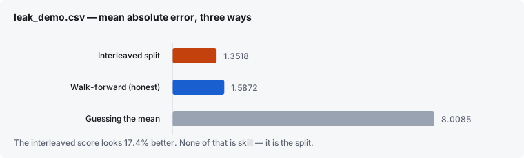
Validation of the indicator. The detector was tested on data whose answer is known in advance. data/leak_demo.csv is a trending, cycling series with lag features $(t-1, t-2, t-3, t-5, t-8)$ plus a row index, constructed so that neighbouring rows carry nearly identical values. With the default seed:
| Regime | Mean absolute error |
|---|---|
| Interleaved split (every 5th row) | 1.3518 |
| Walk-forward (train past, test future) | 1.5872 |
| Guessing the mean | 8.0085 |
Therefore
$$G = 100\,\frac{1.5872 - 1.3518}{1.3518} \approx 17.4\%.$$
Across seeds 1, 42 and 99 the gap measured $+72.2\%$, $+56.2\%$ and $+125.0\%$. The magnitude varies substantially; the sign does not. On files without lag structure the indicator correctly reports no gap.
The strongest check in the suite, and the cheapest.
Targets are randomly permuted across rows while inputs, column ranges and row count are held exactly. Every genuine input–target relationship is destroyed; every structural property of the dataset survives. If $\pi$ is a random permutation,
$$\boxed{\ \mathcal{D}_{\mathrm{shuffled}} = \left\{\left(\mathbf{x}_i,\ \mathbf{y}_{\pi(i)}\right)\right\}_{i=1}^{N}\ } \tag{6.3}$$
An identical network is trained on $\mathcal{D}_{\mathrm{shuffled}}$ and scored identically. The decision rule is:
If the model scores no better on real data than on shuffled data, the score is coming from the procedure, not the data.
Equivalently, a necessary — but not sufficient — condition for useful learned structure is
$$E_{\mathrm{real}} < E_{\mathrm{shuffle}}.$$
If
$$E_{\mathrm{real}} \ge E_{\mathrm{shuffle}},$$
the model has failed the negative control.
This catches what accuracy alone cannot: a leaky split, more parameters than rows can constrain, or a target accidentally reconstructible from the inputs. It is a one-sided test — failing it is conclusive, passing it is not.
On data/powerball_lag.csv, where there is certainly nothing to find:
| Trained on | Validation MSE |
|---|---|
| Real data | $1.767 \times 10^{-1}$ |
| Shuffled targets | $1.731 \times 10^{-1}$ |
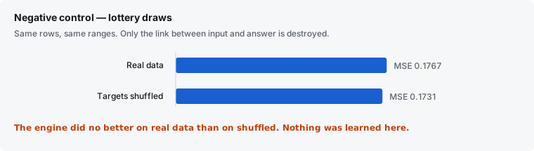
The result is therefore: "The engine did no better on real data than on shuffled."
This is the check to run first on any new file, and the cheapest to run. It needs no domain knowledge, no threshold to argue about, and no judgement call: either the model beats its own sabotaged twin or it does not.
For each input column $c$, that column is permuted across the test rows and the model re-scored. Let $E_0$ be the baseline MAE and $E_{c,r}$ the MAE after the $r$th permutation of column $c$. Then
$$\boxed{\ I_c = \frac{1}{R}\sum_{r=1}^{R}\left(E_{c,r} - E_0\right), \qquad R = 5\ } \tag{6.4}$$
reported in scaled units. A positive $I_c$ means destroying column $c$ makes predictions worse, so the model was using it.
This is measured rather than inferred. Reading weight magnitudes is unreliable: a large weight on a near-constant input contributes nothing, and a small weight on a high-variance input may dominate. A column whose destruction costs nothing was not being used, whatever its weights suggest. But note
$$\boxed{\ \text{importance} \ne \text{causation}.}$$
By default, $M = 5$ networks of identical shape are trained from different random initialisations, seeded by
$$\mathrm{seed}_m = \mathrm{seed} + 7919m.$$
For output $j$, the ensemble mean is
$$\boxed{\ \hat{\mu}_j(\mathbf{x}) = \frac{1}{M}\sum_{m=1}^{M} f_m(\mathbf{x})_j\ }$$
and the ensemble spread is the sample standard deviation
$$\boxed{\ \hat{s}_j(\mathbf{x}) = \sqrt{\frac{1}{M-1}\sum_{m=1}^{M}\left(f_m(\mathbf{x})_j - \hat{\mu}_j(\mathbf{x})\right)^2}\ } \tag{6.5}$$
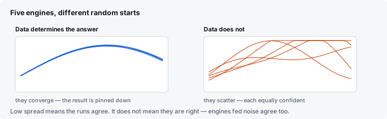
What this is. A measure of how much the answer depends on where optimisation happened to start. Where the data determines the answer, members converge; where it does not, each settles somewhere different while sounding equally confident.
The members need not share a shape. --ensemble accepts a list of architectures, paths to engines saved with --save, or a mixture:
--ensemble 6-5-1,6-12-1,6-8-6-1
--ensemble mymodel.eng,6-5-1
Only the architecture is taken from a saved engine, never its weights: every member must be trained on the same rows, or differences between them would measure their training histories rather than the data. Input and output widths are forced to match the file, since those are fixed by the data rather than chosen.
This widens the question the spread answers. With identical members it measures sensitivity to initialisation — how much the answer depends on where optimisation started. With differing members it measures sensitivity to specification — how much the answer depends on which model was chosen. The second is usually the larger uncertainty and the one that goes unmeasured.
The cost of widening it. A member that simply fits worse will diverge from the others because it is worse, not because the data is ambiguous. Disagreement is evidence about the data only among members that fit comparably well. The software therefore reports each member's held-out error beside the spread, and warns when
$$\frac{\max_m E_m - \min_m E_m}{\tau_{\mathrm{hi}} - \tau_{\mathrm{lo}}} > 0.05,$$
that is, when best and worst span more than 5% of the output range. The test is deliberately expressed against the output range rather than as a ratio $\max_m E_m / \min_m E_m$: when every member fits nearly perfectly the smallest error approaches zero and the ratio diverges to an arbitrarily large multiple while the members are in fact indistinguishable.
What this is not. It is not a confidence interval and not a probability. It carries no information about whether the converged answer is correct — only about whether it is determined. Networks trained on pure noise agree with each other too, because they all converge to the mean. Formally,
$$\boxed{\ \text{low ensemble spread} \not\Rightarrow \text{high accuracy}.}$$
The model card states this explicitly: stable is not the same as correct.
Mean squared error is
$$\boxed{\ \mathrm{MSE} = \frac{1}{N}\sum_{i=1}^{N}\sum_{j=1}^{n_{\mathrm{out}}}\left(f_j(\mathbf{x}_i) - y_{ij}\right)^2\ } \tag{6.6}$$
Mean absolute error is
$$\boxed{\ \mathrm{MAE} = \frac{1}{N n_{\mathrm{out}}}\sum_{i=1}^{N}\sum_{j=1}^{n_{\mathrm{out}}}\left|f_j(\mathbf{x}_i) - y_{ij}\right|\ } \tag{6.7}$$
MSE is computed in scaled units and used for model selection, since it is the quantity being optimised. MAE is denormalised via (2.3) and reported in the user's real units, since it is the quantity a person can interpret.
Implementation note for validation. The asymmetry between (6.6) and (6.7) is real and has been verified against the source, not inferred. meanSquaredError sums squared error over output columns and divides by the row count alone, while meanAbsError divides by the total element count $N n_{\mathrm{out}}$. The two metrics therefore differ by a factor of $n_{\mathrm{out}}$ beyond the square-versus- absolute distinction, so their magnitudes are not comparable when $n_{\mathrm{out}} > 1$.
This does not affect any reported conclusion, because MSE is used only to rank candidate shapes against one another on the same dataset, where the constant $n_{\mathrm{out}}$ cancels. It would matter if an MSE figure were compared across files with different output counts, and it is documented here so that no reader does so by accident.
Two naive baselines are used. The mean baseline is
$$\hat{\mathbf{y}} = \mathrm{mean}(\mathbf{y}_{\mathrm{train}}),$$
reported by --auto. The no-change baseline at forecast horizon $h$ is
$$\boxed{\ \hat{y}_t^{\,\mathrm{NC}} = y_{t-h}\ }$$
scored as
$$\boxed{\ \mathrm{MAE}_{\mathrm{NC}}(h) = \frac{1}{N-h}\sum_{t=h+1}^{N}\left|y_t - y_{t-h}\right|\ }$$
and reported by --ticker. The baseline therefore says "the series has not moved over the interval you are trying to forecast" — not merely lag-one persistence.
The no-change baseline is the demanding one for time series. Beating the mean on a trending series is trivial; beating last-known-value is not.
--stream predicts each case before training on it. At time $t$,
$$\boxed{\ \hat{\mathbf{y}}_t = f_{t-1}(\mathbf{x}_t)\ }$$
is recorded before the update
$$\boxed{\ f_t = \mathrm{Update}\!\left(f_{t-1}, \mathbf{x}_t, \mathbf{y}_t\right).\ }$$
The information order is therefore
$$\boxed{\ \text{Predict}_t \;\longrightarrow\; \text{Observe } \mathbf{y}_t \;\longrightarrow\; \text{Train}_t\ }$$
rather than $\text{Train}_t \longrightarrow \text{Predict}_t$.
Every prediction is made using only information available at that time. This is the distinction between prequential evaluation and a backtest: no retrospective refitting is possible, because the model at step $t$ has never seen step $t+1$.
Scaler bounds are widened, not refitted, when a value arrives outside the observed range (expandToInclude). Refitting would move every column's scale simultaneously and invalidate what the weights had learned; widening only where the data actually went keeps the mapping stable and monotonic.
All randomness derives from a single user-settable seed (--seed): weight initialisation, target shuffling for the negative control, column permutation for importance, and ensemble member offsets. Fixing the seed makes a run bit-for-bit reproducible.
--save writes the topology and every weight. A saved engine reloads already trained. This matters because a result that cannot be reproduced three months later is a story about a result, not a result.
The preceding sections describe checks that make self-deception harder. None of them make it impossible, and the following limitations are structural rather than implementation defects.
No method establishes future performance. Walk-forward, negative controls, permutation importance and ensemble agreement together substantially raise the difficulty of fooling yourself. They say nothing about whether a relationship found in historical data will persist. Conditions change and relationships break down; a model passing every check here may still fail in use.
The leak indicator is one-sided. A large gap proves the interleaved score was inflated. A small gap proves only that this particular leakage mechanism was not operating. It does not rule out target leakage from a feature computed using future information, survivorship bias in row selection, or a target revised after the fact. The software cannot detect those and does not claim to.
The negative control is one-sided. Failing it is conclusive: the score came from procedure, not data. Passing it establishes only that the model beats a destroyed-relationship version of itself, which is a low bar.
Ensemble spread measures determinacy, not accuracy. See Section 6.6. Agreement among members trained on noise is expected, not reassuring.
Permutation importance measures use, not causation. It reports what the model relied on. A model relying heavily on a spurious correlate will show that correlate as important. Importance is a fact about the model, not about the world.
Beating a baseline is not profitability. If the engine beats a naive baseline, the model carries information the baseline lacks. Transaction costs, spreads, slippage, liquidity, taxes, timing and execution are modelled nowhere in this software and appear in none of its figures.
Results depend entirely on supplied data. Data that is incomplete, mislabelled, revised after the fact, survivorship-biased, or that leaks future information into the past will produce results that look valid and are not. Most of these conditions are undetectable from the file alone.
The optimiser is plain SGD with momentum. There is no adaptive learning rate, batch normalisation, or dropout. Regularisation is weight decay plus the capacity budget in Section 5. This is a deliberate scope decision — the engine exists to be inspectable, and every quantity above can be checked by hand — but it means the engine is not competitive with a modern gradient-boosted tree on tabular data, and does not claim to be. The verification layer, not the engine, is the product.
The central caution can be stated symbolically as
$$\boxed{\ \text{Passing all checks} \not\Rightarrow \text{future correctness}.}$$
| Parameter | Default | Set by |
|---|---|---|
| Learning rate $\eta$ | 0.5 | --lr |
| Momentum $\mu$ | 0.9 | --momentum |
| Bias activation $\beta$ | 0.5 | fixed |
| Output delta cap $\Delta$ | 1.0 | fixed |
| Step cap $S$ | 1.0 | fixed |
| Weight decay $\lambda$ | 0 in batch; on in streaming | mode-dependent |
| Target band | $[0.1, 0.9]$ | fixed |
| Weights per row $\rho$ | 3 | --weights-per-row |
| Iterations $T$ | Equation (5.2) | --iterations |
| Walk-forward folds $F$ | 3 | fixed |
| Interleaved $k$ | 5 | fixed |
| Ensemble members $M$ | 5, all the chosen shape | --ensemble |
| Output activation | Chosen from data | --linear / --sigmoid |
DetectBS --auto --in data/powerball_lag.csv
    # Section 6.4 negative control

DetectBS --auto --leak-check --in data/leak_demo.csv
    # Section 6.3 leak indicator

DetectBS --auto --leak-check --seed 42 --in data/leak_demo.csv

DetectBS --auto --in data/t_signal.csv --ensemble 3-1,3-20-1,3-16-12-1
    # Section 6.6 user-defined ensemble members, and the
    # comparability warning when they do not fit equally well

DetectBS --ticker
    # Section 6.7 no-change baseline

DetectBS --stream --inputs N
    # Section 7 prequential evaluation
Sample data ships with the software. Figures quoted in Sections 2 and 4 are from the development record and are reproducible from the same files at the stated iteration counts.
Detect BS is a tool for evaluating models. It is not financial, investment or professional advice. © 2026 Micah Forstein.